Statistics

Basic Statistics

Formulas

1. Pearson’s first coefficient of skewness, or Pearson mode skewness

(1) $\begin{equation*} S_k1 = \frac{(\bar{X} - M_o)}{\sigma}\end{equation*}$

2. Pearson’s second coefficient of skewness, or Pearson median skewness

(2) $\begin{equation*} S_k2 = \frac{3*(\bar{X} - Med)}{\sigma}\end{equation*}$

$\bar{X}$ : Mean

$M_o$ : Mode

$Med$ : Median

$\sigma$ : Standard Deviation

Common Terminologies

Data or Raw Data or Ungrouped Data

Two types of Raw Data – Primary Data and Secondary Data. The raw data is put in tabular form for further analysis. Data arrangement can be done in Alphabetical/Ascending/Descending order.

Primary Data or First-Hand Data

Investigators collect the data by themselves with a definite plan or design

Secondary Data

Investigators don’t collect it themselves but obtain it from published or unpublished sources. Secondary data collected by an individual or institution for some purpose, & are used by someone else in another context.

Array or Arrayed Data

Raw data is put in ascending or descending order of magnitude.

Observation

Each data entry in the table is called an observation

Frequency

Number of times a particular observation occurs in a given set of data.

Skewed Data

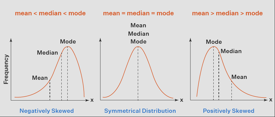
Skewed data creates an asymmetrical, skewed curve on a graph. The normal distribution is symmetrical (zero skew value) and shaped like a bell. But a lognormal distribution would exhibit some right skew.

However, skewed data has a “tail” on either side of the graph. Most real-world situations aren’t symmetrical—real data sets are usually skewed. The two most common types of skew are:

Negative skew: A data set with a negative skew has a tail on the negative side of the graph, meaning the graph is skewed to the left. In this case, mean < median < mode
Positive skew: A data set with a positive skew has a tail on the positive side of the graph, meaning the graph is skewed to the right. In this case, mean > median > mode

How to calculate skewness

Skewness is the degree of asymmetry observed in a probability distribution. Skewness tells us where the outliers occur, although it doesn’t tell you how many outliers occur.

There are several ways to measure skewness. Pearson’s first and second coefficients of skewness are two common methods.

Pearson’s first coefficient of skewness, or Pearson mode skewness, subtracts the mode from the mean and divides the difference by the standard deviation.

Sk1 = (mean – mode) / standard deviation

Pearson’s second coefficient of skewness, or Pearson median skewness, subtracts the median from the mean, multiplies the difference by three, and divides the product by the standard deviation.

Pearson’s first coefficient of skewness is useful if the data exhibit a strong mode. If the data have a weak mode or multiple modes, Pearson’s second coefficient may be preferable, as it does not rely on mode as a measure of central tendency.

Problem with the skewed data

Many statistical models don’t work effectively with skewed data. Outliers adversely affect a model’s performance, especially regression-based models. While there are statistical models that are robust enough to handle outliers like tree-based models, you’ll be limited in what other models you can try. So what do you do? Removing outliers and normalizing our data will allow us to experiment with more statistical models.

Transform your skewed data

Depending on your dataset, we can choose to transform skewed data to Gaussian (or normal) distribution through techniques like:

Exponential transformation: Involves using exponents to transform a data set from skewed to normal distribution.
Power transformation: Involves using functions to make a data set closer to normal distribution.
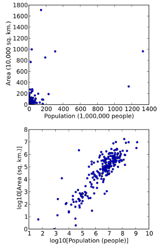
Log transformation: Involves using the natural log to make a data set closer to normal distribution. Log Transformation is a data transformation method in which we apply a logarithmic function to the data. It replaces each value x with log(x). After log transformation, we can see patterns in our data much more easily

Skewed data examples

Positive skew example

One example of positively skewed data could be a typical income data set. If we draw a curve of a sample population’s income on a graph, the curve is likely to be skewed to the right, or positively skewed. This would occur if most people have average incomes, and a smaller number of people have high incomes. The people with high incomes would be the outliers in the data set that skew the curve toward the right side of the graph.

Negative skew example

An example of negatively skewed data could be the exam scores of a group of college students who took a relatively simple exam. If we draw a curve of the group of students’ exam scores on a graph, the curve is likely to be skewed to the left. In this case, most students would have high test scores, and a smaller number of people would have low scores that skew the curve toward the left of the graph. The students with the lower scores would be the outliers in the data set causing it to be negatively skewed.