Percentiles and Moments

Introduction

Statistical measures like percentiles and moments are crucial in understanding data distributions.

• Percentiles describe the relative standing of a data point in a dataset.
• Moments capture various aspects of a distribution such as centrality, spread, skewness, and kurtosis.

These concepts are widely used in descriptive statistics, machine learning, risk analysis, and anomaly detection.

1. Percentiles

Definition

A percentile is a measure that indicates the value below which a given percentage of observations fall. The p-th percentile of a dataset is the value below which p% of the data lies.

Mathematical Formula

For a dataset of size N, the percentile rank of the i-th observation  is given by:

where:

• $i$ is the index of the sorted data,
• $N$ is the total number of observations.

Common Percentiles in Data Science

• 25th percentile (Q1) → First Quartile
• 50th percentile (Q2) → Median
• 75th percentile (Q3) → Third Quartile
• 90th percentile → Often used in performance analysis
• 99th percentile → Detecting anomalies
• IQR (Interquartile Range) -> is a measure of statistical dispersion or spread in a dataset. It represents the range between the first quartile (Q1) and the third quartile (Q3), essentially capturing the middle 50% of the data. i. e IQR=Q3−Q1

  Where:

  • Q1 (the first quartile) is the median of the lower half of the dataset (25th percentile).
  • Q3 (the third quartile) is the median of the upper half of the dataset (75th percentile).

  How to calculate it:

  1. Sort the data in increasing order.
  2. Find Q1: This is the median of the lower half of the data (the data points below the overall median).
  3. Find Q3: This is the median of the upper half of the data (the data points above the overall median).
  4. Calculate the IQR: Subtract Q1 from Q3.

Example in Data Science

• Outlier Detection: Any value beyond the 1.5 × IQR (Interquartile Range) is considered an outlier.
• Machine Learning Model Evaluation: Percentiles help in benchmarking model performance (e.g., latency, error rates).

Python Example of Percentile Calculation

import numpy as np

# Sample data (response times in ms)
data = np.array([10, 20, 22, 30, 35, 40, 50, 55, 60, 100])

# Compute percentiles
percentiles = [25, 50, 75, 90, 99]
values = np.percentile(data, percentiles)

# Display results
for p, v in zip(percentiles, values):
    print(f"{p}th percentile: {v}")

#Output
#25th percentile: 24.0
#50th percentile: 37.5
#75th percentile: 53.75
#90th percentile: 63.999999999999986
#99th percentile: 96.4

2. Moments in Statistics

Definition

In statistics, moments are quantitative measures that describe the shape of a probability distribution.

There are four main moments:

1. First Moment (Mean) → Measures central tendency
2. Second Moment (Variance) → Measures spread
3. Third Moment (Skewness) → Measures asymmetry
4. Fourth Moment (Kurtosis) → Measures tail heaviness

1st Moment: Mean

The mean \mu is the average of all observations:

data_mean = np.mean(data)
print(f"Mean: {data_mean}")

2nd Moment: Variance (Spread of Data)

Variance \sigma^2 measures data dispersion:

data_variance = np.var(data)
print(f"Variance: {data_variance}")

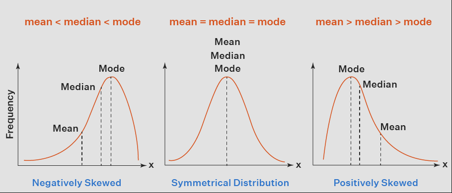
3rd Moment: Skewness (Asymmetry of Data Distribution)

Skewness tells whether a distribution is left-skewed (negative), symmetric (zero), or right-skewed (positive).

• Positive Skew: Right tail is longer (e.g., income distribution).
• Negative Skew: Left tail is longer (e.g., exam scores).

from scipy.stats import skew

data_skewness = skew(data)
print(f"Skewness: {data_skewness}")

4th Moment: Kurtosis (Tail Heaviness)

Kurtosis measures whether data has heavy or light tails compared to a normal distribution.

• High Kurtosis (>3): More outliers, heavy tails (e.g., stock market returns).
• Low Kurtosis (<3): Fewer extreme values, light tails (e.g., uniform distribution).

from scipy.stats import kurtosis

data_kurtosis = kurtosis(data)
print(f"Kurtosis: {data_kurtosis}")

How Percentiles and Moments Are Used in Data Science?

1. Feature Engineering:

   • Percentiles help normalize data and detect outliers.
   • Moments help extract important distribution characteristics for modeling.

2. Anomaly Detection:

   • High kurtosis and extreme percentiles can signal outliers in datasets.

3. Machine Learning Model Evaluation:

   • Percentiles (e.g., 90th percentile latency) measure model efficiency.
   • Variance & Skewness help understand dataset imbalance.

4. Risk Analysis in Finance:

   • Percentiles are used in Value at Risk (VaR) models.
   • Moments (Kurtosis & Skewness) help assess stock return distributions.

Detecting Outliers Using Percentiles & Moments

import matplotlib.pyplot as plt

# Generate a dataset with outliers
np.random.seed(42)
data = np.random.normal(50, 10, 1000)  # Normal distribution
data = np.append(data, [150, 200, 250])  # Adding outliers

# Compute percentiles
Q1, Q3 = np.percentile(data, [25, 75])
IQR = Q3 - Q1
lower_bound = Q1 - 1.5 * IQR
upper_bound = Q3 + 1.5 * IQR

# Detect outliers
outliers = data[(data < lower_bound) | (data > upper_bound)]
print(f"Detected outliers: {outliers}")

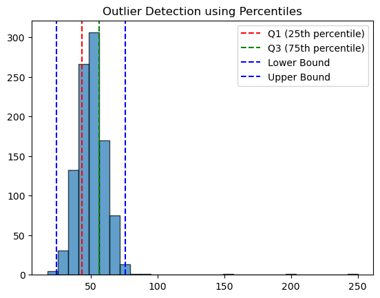
# Plot data distribution
plt.hist(data, bins=30, edgecolor='black', alpha=0.7)
plt.axvline(Q1, color='r', linestyle="--", label="Q1 (25th percentile)")
plt.axvline(Q3, color='g', linestyle="--", label="Q3 (75th percentile)")
plt.axvline(lower_bound, color='b', linestyle="--", label="Lower Bound")
plt.axvline(upper_bound, color='b', linestyle="--", label="Upper Bound")
plt.legend()
plt.title("Outlier Detection using Percentiles")
plt.show()